Primer for Data Analysis Tools

A primer on MS/MS analysis tools at the UWPR

Analysis software overview

The two primary analyses performed at the UWPR are shotgun (bottom-up) proteomics and targeted quantitative proteomics.

For targeted proteomics, data is classically acquired on triple quadrupole instruments and typically analyzed using the Skyline software suite. There is extensive documentation on the Skyline website, along with tutorials and videos.

Shotgun analysis involves peptide identification via MS/MS database searching. Popular commercial tools are Thermo’s Proteome Discoverer and Proteome Software’s Scaffold. Free tools such as MaxQuant and FragPipe are widely used for peptide identification, quantification, and more.

To use the same tools we use here at the UWPR, you can learn about the Trans-Proteomic Pipeline (TPP), originally developed in the Aebersold group at ISB. There is a support forum for your questions.

Getting to your processed data (UWPR users only)

Shotgun data processed by the UWPR for you will typically entail a Comet database search followed by Trans-Proteomic Pipeline (TPP) analysis using PeptideProphet (Ref 1) and ProteinProphet (Ref 2). Aimed at someone new to UWPR proteomics analysis, this is a brief tutorial on how to start looking at your data.

Links to your processed data appear at the bottom of your project page in the section “External Links to Data”.

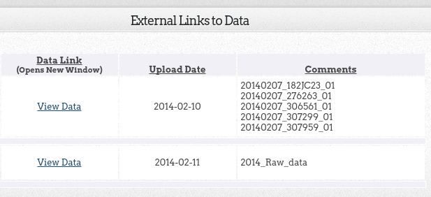
Click on the “View Data” link, which brings up a page that looks like this:

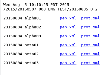
Clicking on these links will prompt you to authenticate again using the same user name and password that gets you into your UWPR project page. If you are sure you are using the same login credentials but still cannot access the data links, contact us.

Checking PeptideProphet score distributions

The very first thing I always look at is PeptideProphet’s score distribution plots and how well the modeled positive and negative distributions fit the experimental data. To do this, click on the “pep.xml” file link for each analysis. This brings up the TPP’s PepXML Viewer below. Think of it as a grid of your raw search results where each row represents an MS/MS spectrum search result. You will see some scores, a spectrum name with the scan number and charge state encoded in it, a link to the spectrum viewer, the best (not necessarily correct) peptide match, a protein name (just one protein name is printed, but the peptide could match many), and the peptide mass. You can add or remove other columns of information.

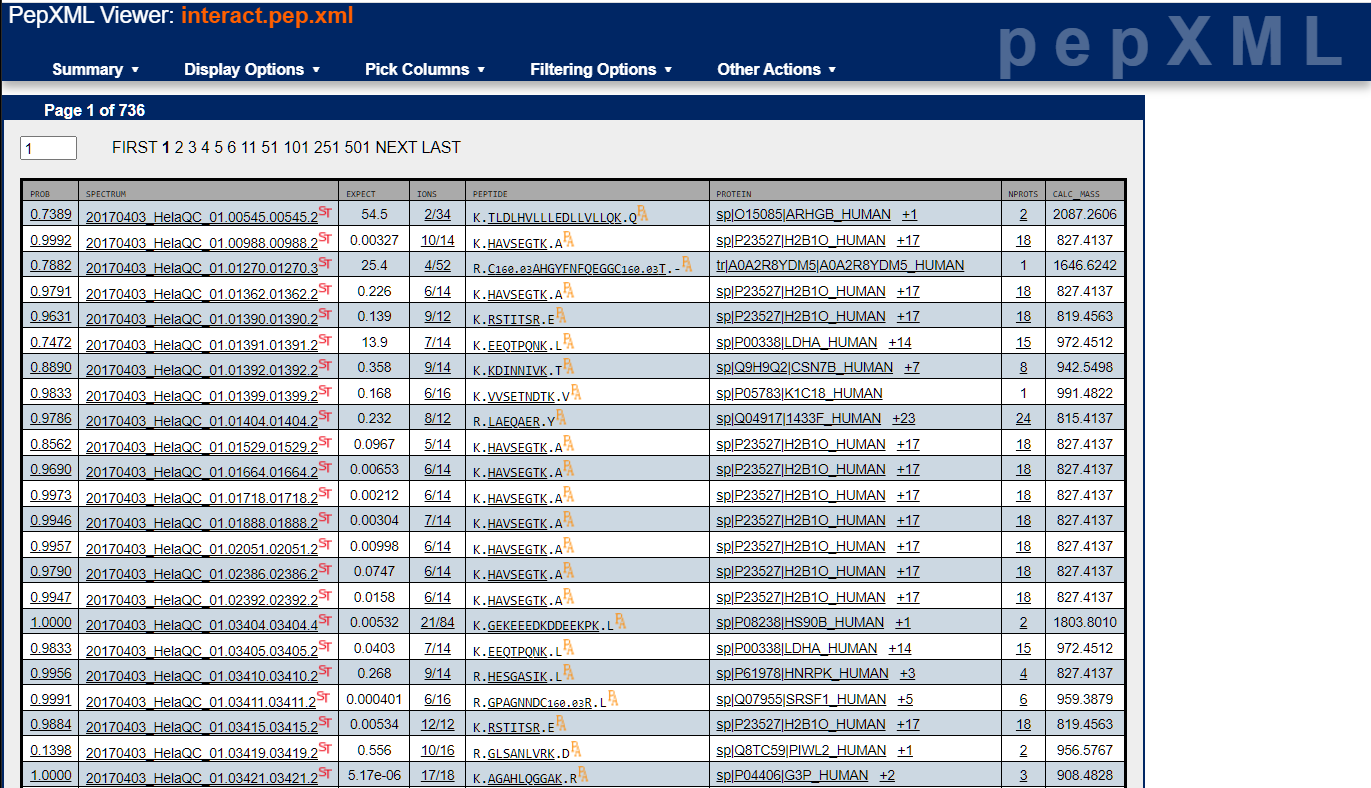
Then click on any of the probability score values in the leftmost column with the header “PROB”. They all bring up the same score distribution curves, so it does not matter which one you click on. You should see a set of model charts like the ones below. There is a lot of information here that is beyond this primer; your best resource for questions on PeptideProphet and these score distributions is the TPP’s support forum.

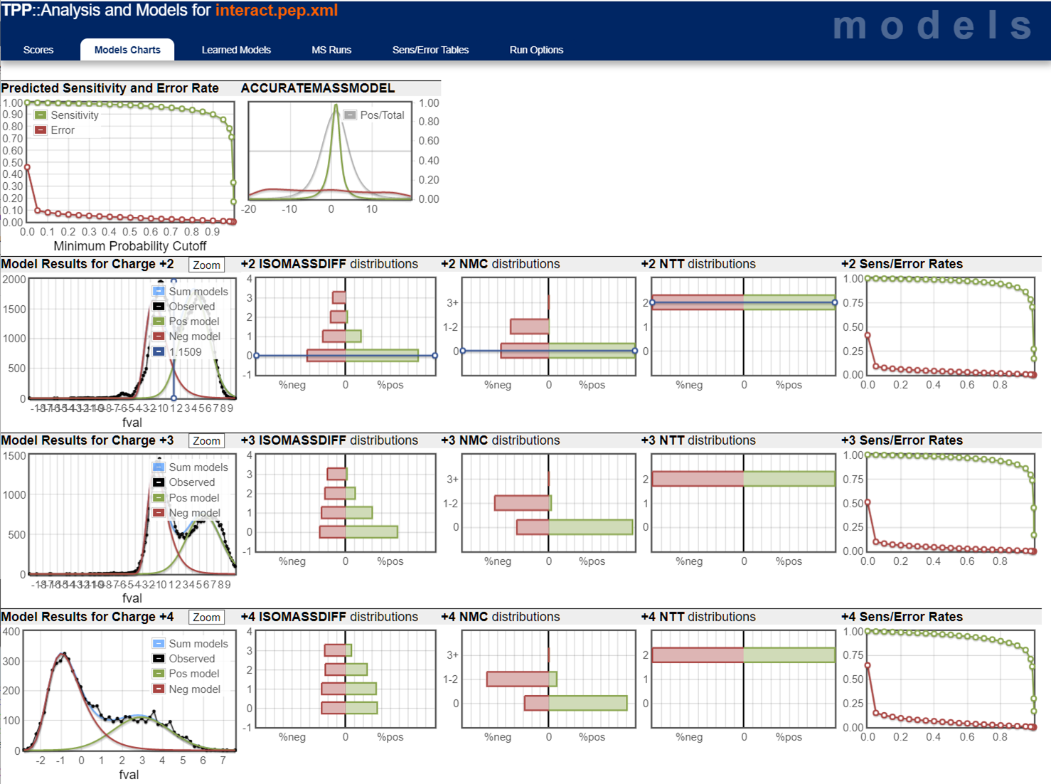
The charts on the far left are the key indicators and what I use to judge whether or not the calculated probability values are worthwhile.

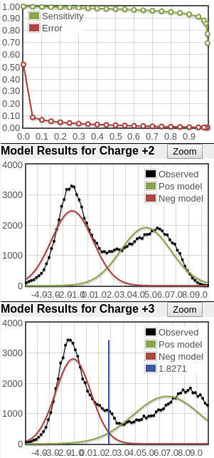
What you see in the plots is a score histogram (black curves) of all the peptide identifications, one plot for each precursor charge state. The red curves are what PeptideProphet fits to the negative/null/wrong distribution, and the green curves are what PeptideProphet fits to the positive/correct distribution. What you want to see is two distinct distributions (bimodal) in the black curve, with the red and green curves fitting them well. Note: although each peptide-spectrum match has a link to the model charts, they all point to the same set of curves; the only difference is the score mark for the specific PSM.

Here are two examples of very good score distributions. The sensitivity/error curves are near ideal (you want them to hit the top right and bottom left corners). The black line in the second and third plots represents the histogram of search results, and you want to see a bimodal (two peak) distribution representing the bad hits (modeled by the red curve) and the good hits (modeled by the green curve). In these examples, it is clear that there are two peaks in the black score distribution and the positive distributions are big.

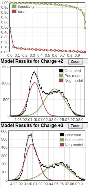
Here are two examples of other good, perhaps more typical distributions. The positive distributions are not nearly as large as in the plots above, but they are clear positive distributions. In the plots on the right, the lines are jagged simply because the raw counts are so low. But even with these low counts, there is good separation between the positive and negative distributions (and this good separation is encapsulated in the good sensitivity/error plots).

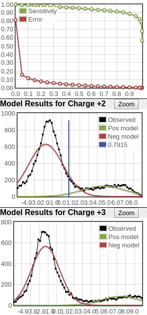
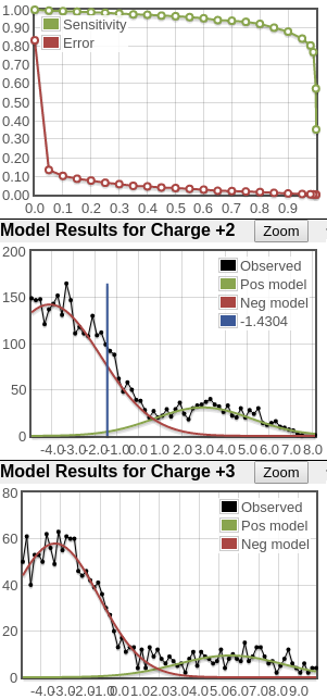
Here is an example of very poor score distributions. The sensitivity/error plots do not trend to the top right and bottom left corners, and there is simply no positive distribution. So if there are any good peptide IDs, their counts are very low.

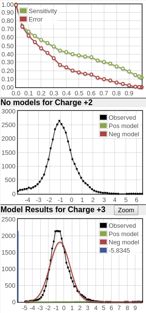
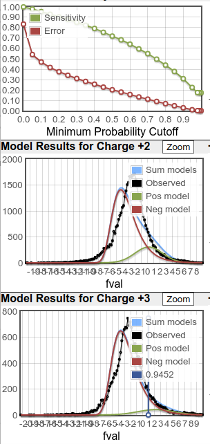
When the score distributions are as poor as in the third example above, I tend to ignore the calculated probability values, which means the protein probabilities are not reliable either (do not bother opening the prot.xml link). For such data, I end up sorting the peptide list in ascending order by the “expect” column (E-value or expectation value) and looking at the best scoring identifications. In contrast to PeptideProphet probabilities, which are calculated by analyzing the entire run, the E-value is calculated on each individual spectrum search; smaller E-values are better. Think of it as related to a p-value, but with the definition that it is the expected number of random identifications that score as well as or better than the current peptide’s score. By observation of Comet scores and the spectral annotations, E-values in the range of 10^-8 or smaller are usually very good, while spectra with scores in the 10^-4 range and higher start to look more noisy and suspect. And there are always exceptions (like a good looking spectrum match with a poorer E-value). Note that there is an issue where extremely poor matches of, say, a single fragment ion can generate low E-values, so always glance at the “IONS” column as well; any entries with just 1 or 2 fragment matches, e.g. “1/20”, indicate a poor match.

Filtering by false discovery rate

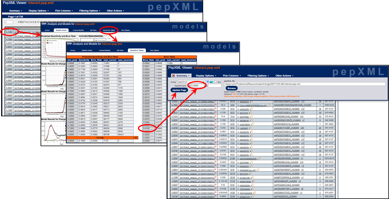
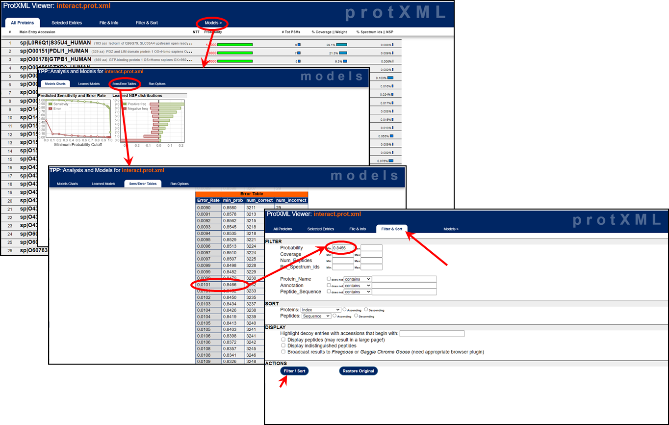
Both the pep.xml and prot.xml viewers allow you to filter the data. For example, in order to target a specific false discovery rate, you can look up the appropriate probability score cutoff. In the pep.xml viewer, click on any probability score and then click on “Sens/Error Tables”. Look at the “Error Table” and the “Error_Rate” column, which represents the false discovery rate. If you want to filter the results at a 1% or a 5% false discovery rate, find the “min_prob” minimum probability that corresponds to the 0.01 or 0.05 “Error_Rate” value. Now you can filter your results with this minimum probability cutoff to target your specific false discovery rate. (Use the global error rate values and ignore those specific to each charge state.) Click on the images below for a larger view of the filtering workflows.

pep.xml FDR filtering: prot.xml FDR filtering:

Viewing annotated spectra

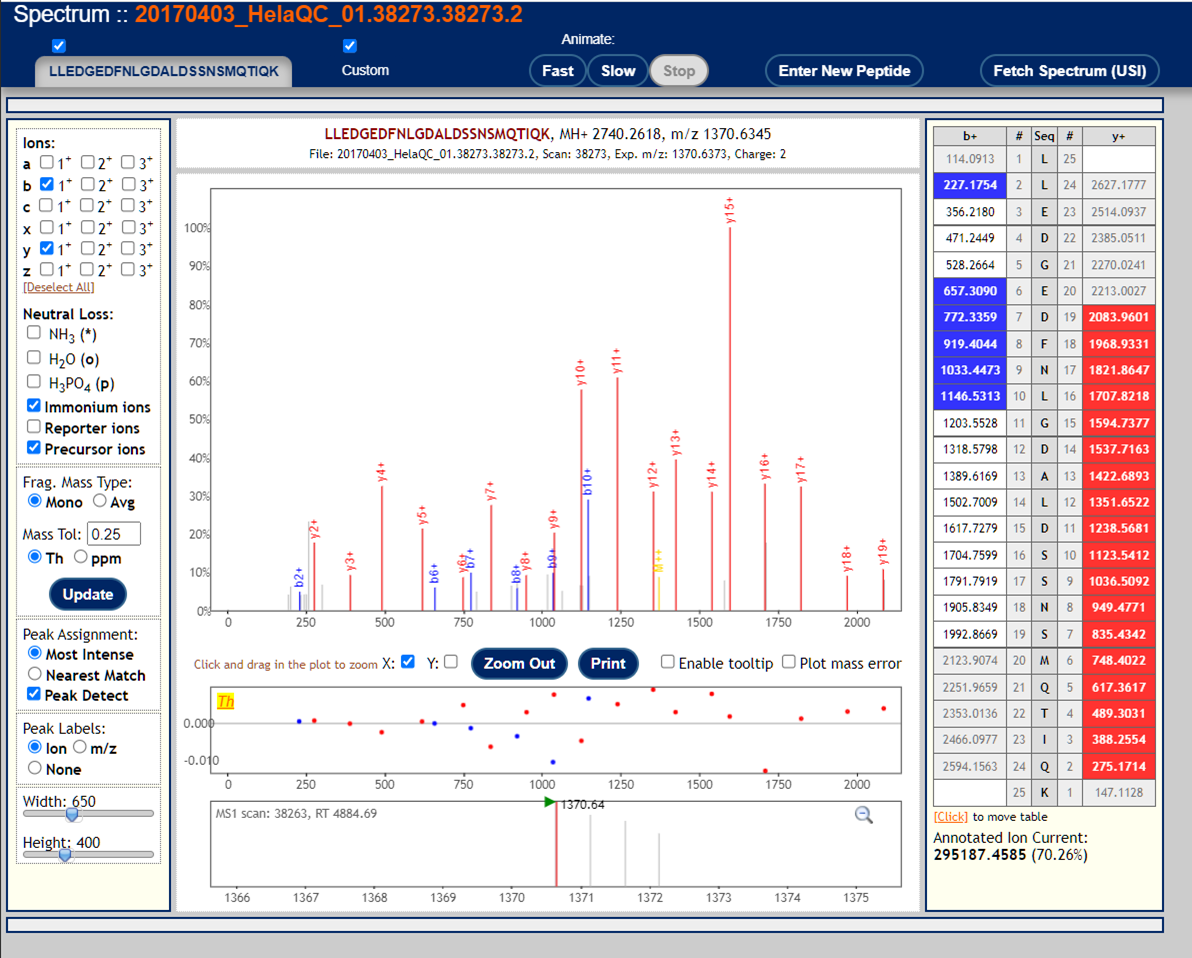
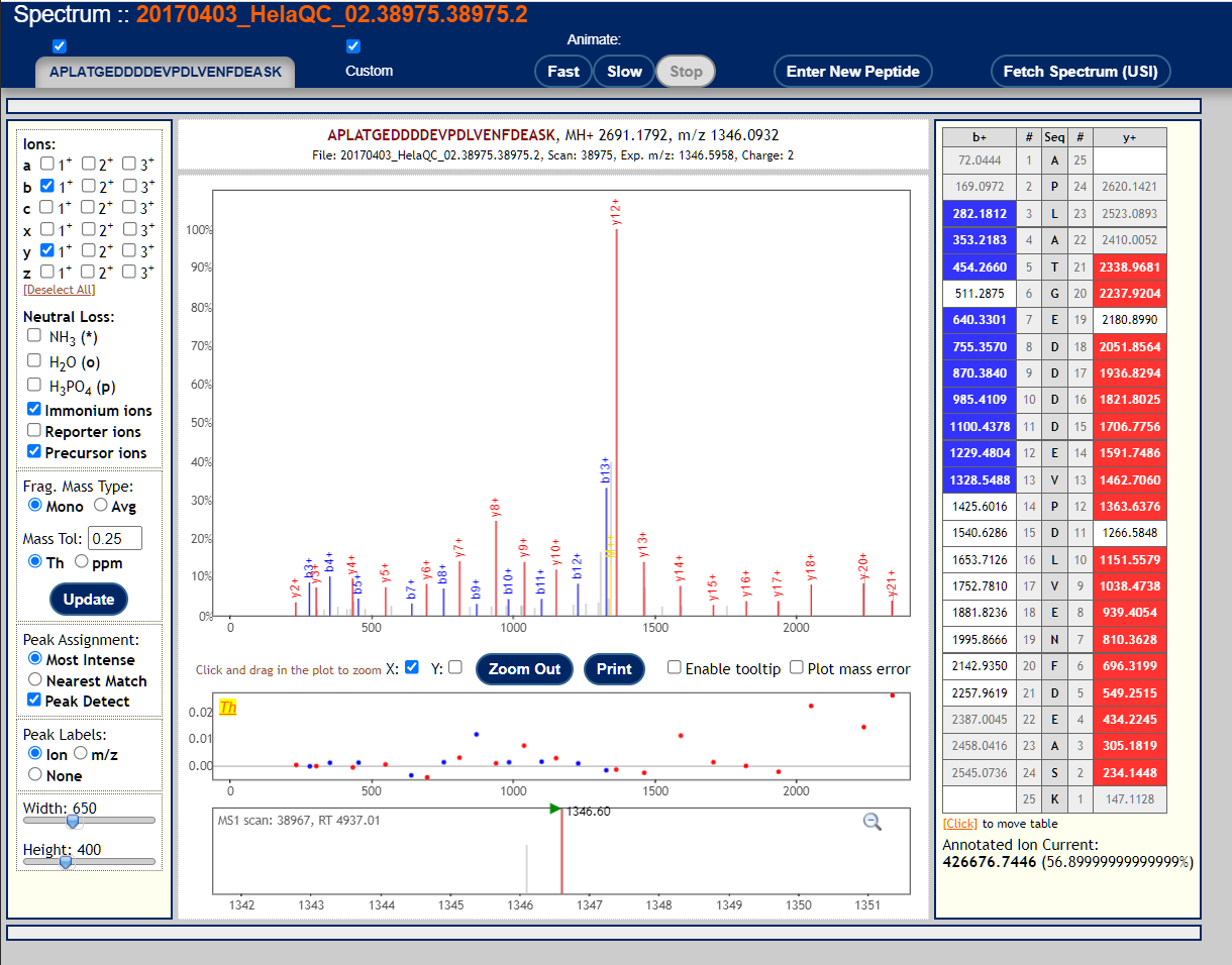
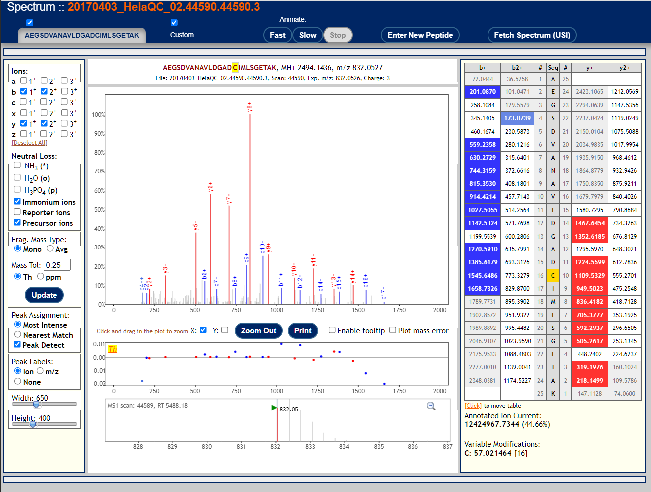
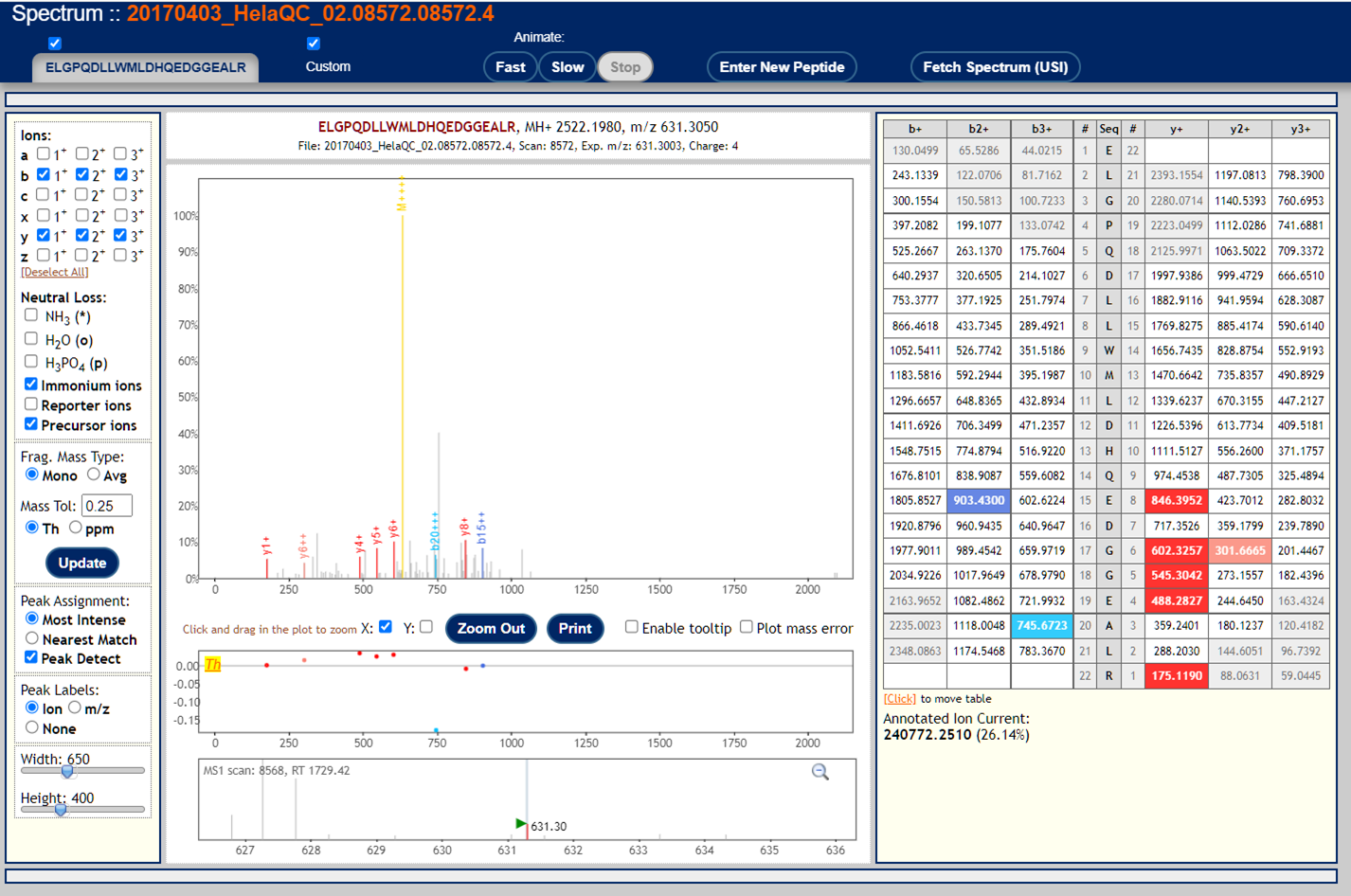
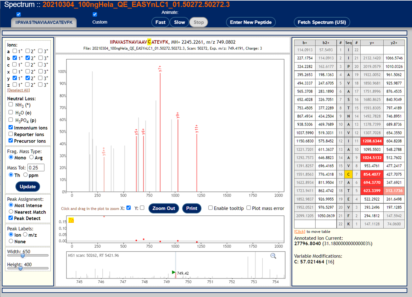
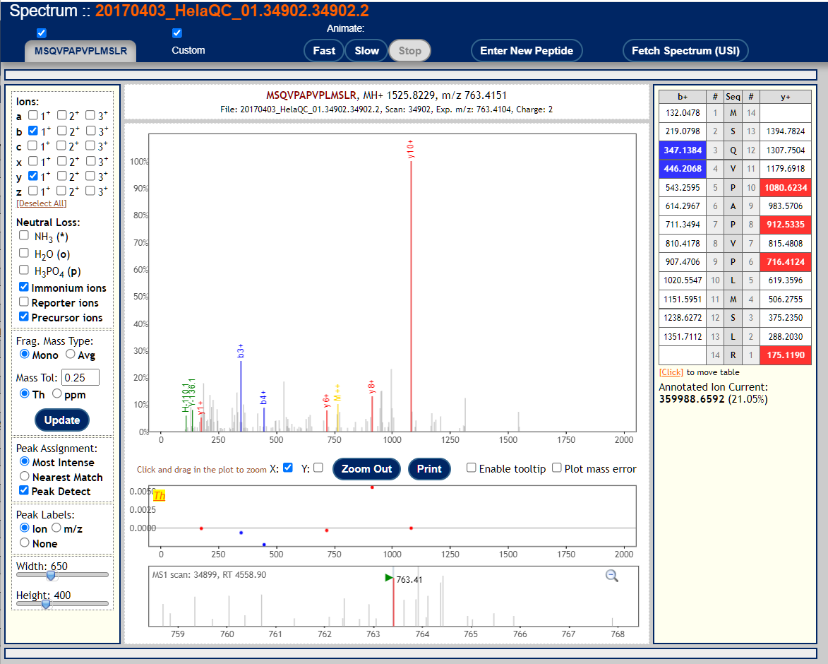
To visualize annotated spectra using the Lorikeet viewer, click on the links in the “IONS” column of the PepXML Viewer. Here are three examples of good MS/MS spectra with good peptide matches.

These are examples of very poor MS/MS spectra.

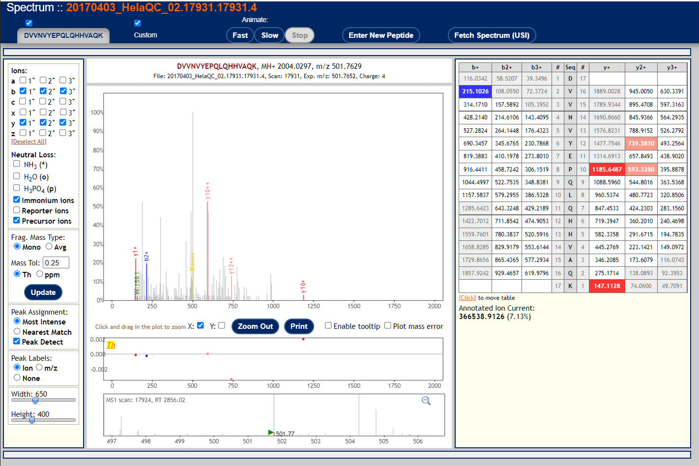
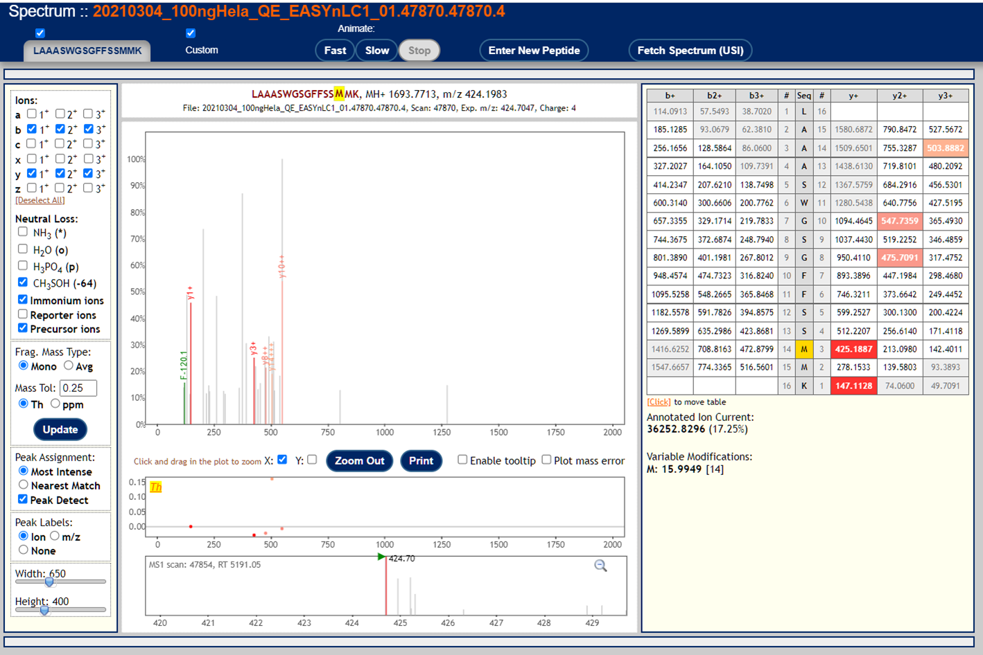
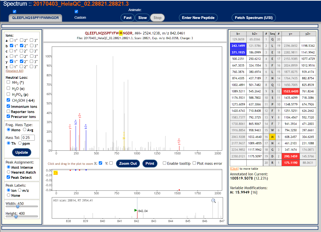
These peptide-spectrum matches got poor scores but might seem plausible if you squint your eyes hard enough. This reflects the fact that mass spectra are not binary (correct/incorrect) data, so identifications and identification confidence are also not black and white.

Protein-level results

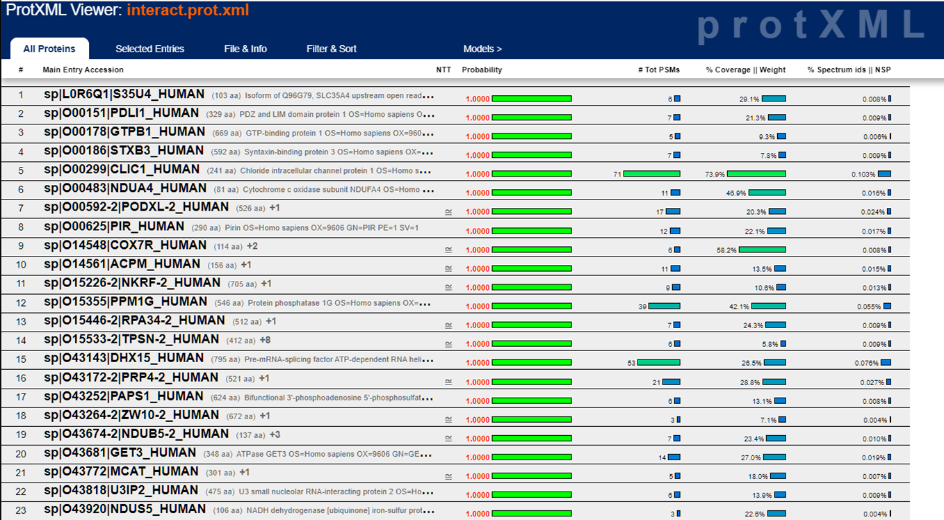
The prot.xml link brings up the ProteinProphet viewer. This is a protein centric view of the data and should only be looked at after you validate that the peptide score distributions are not horrible. Here is what the ProteinProphet viewer looks like:

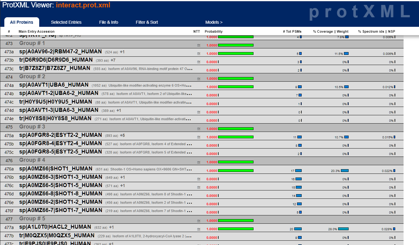
Scrolling down the list, you start seeing protein “groups”, which are usually isoforms grouped together (but sometimes they are unrelated proteins that simply share sequence homology):

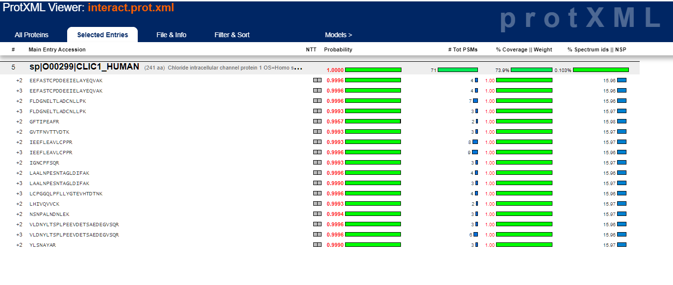
Clicking on the far left column for a particular protein entry brings up these peptide details:

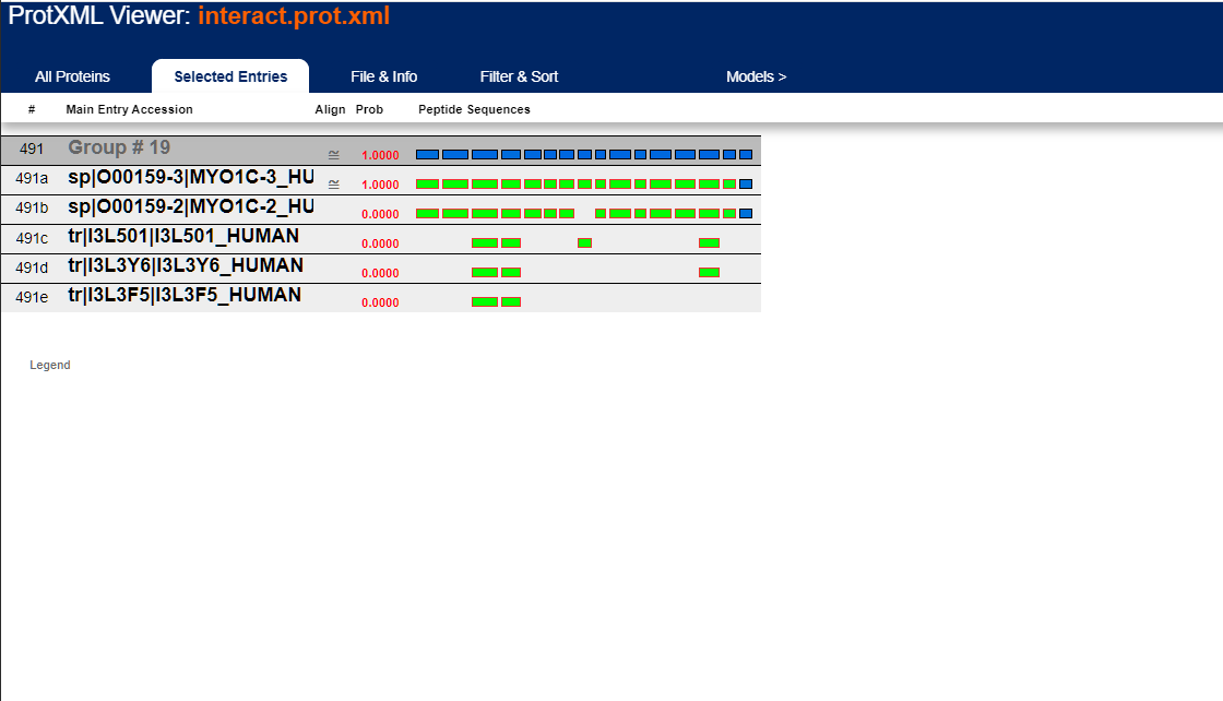
Clicking on the group entry number brings up the group details below, where the shaded boxes represent peptide IDs across the proteins in the group. As you can see, entry “sp|O00159-3|MYO1C-3_HUMAN” contains every peptide identified across this set of 5 proteins, whereas the other 4 proteins match a subset of those peptides. This is why “sp|O00159-3|MYO1C-3_HUMAN” has a probability of 1.0000 while the other 4 proteins have a probability of 0.0000. This does not mean that the other proteins are not present in your sample; there is no way to know this from the peptide data. The ProteinProphet software apportions the probability values across the simplest list of proteins that can explain the identified peptides, which in this case is that single protein entry; that is simply the convention its authors decided to take. All 5 proteins are still part of the protein group, and any or all of them might be present irrespective of the individual assigned protein probabilities.

Exporting spreadsheets

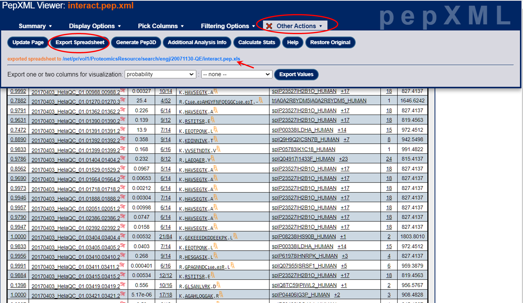
For the pep.xml link, after you choose “Export Spreadsheet”, go back to the “Summary” tab. In the header, you should now see an “exported spreadsheet to:” text with a hypertext link to the .xls file (which is really just a tab-delimited text file); see the image below. Click on the link to download the .xls file and open it in Excel.

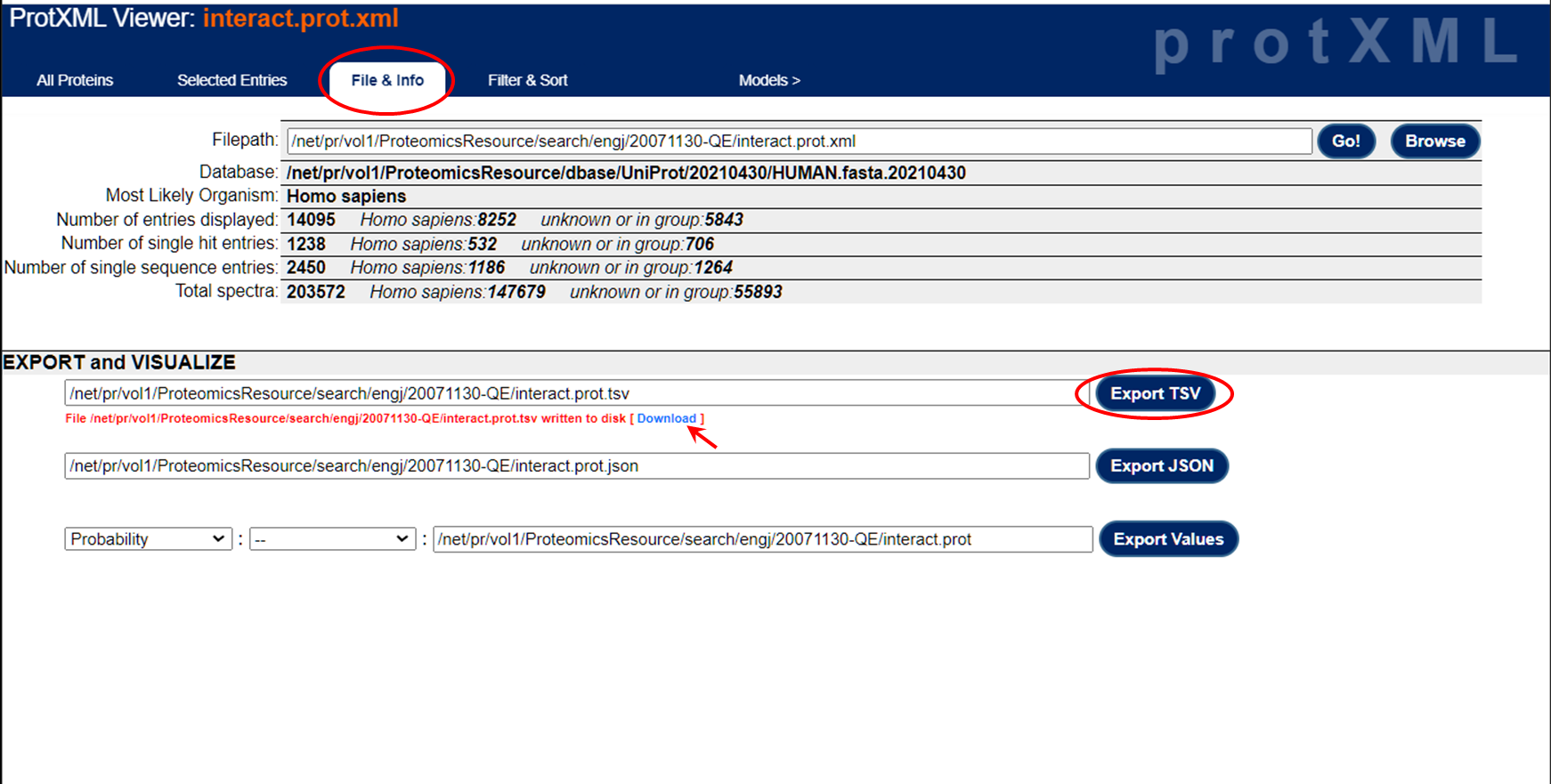
It is a little more convoluted to get the exported file from the prot.xml view. Once you hit the “Export to XLS” button in the protein view, you end up with something like this:

TMT and iTRAQ quantification (Libra)

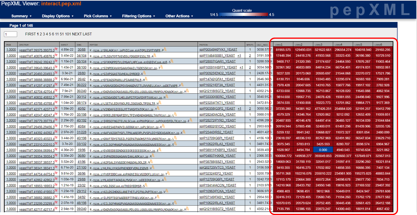
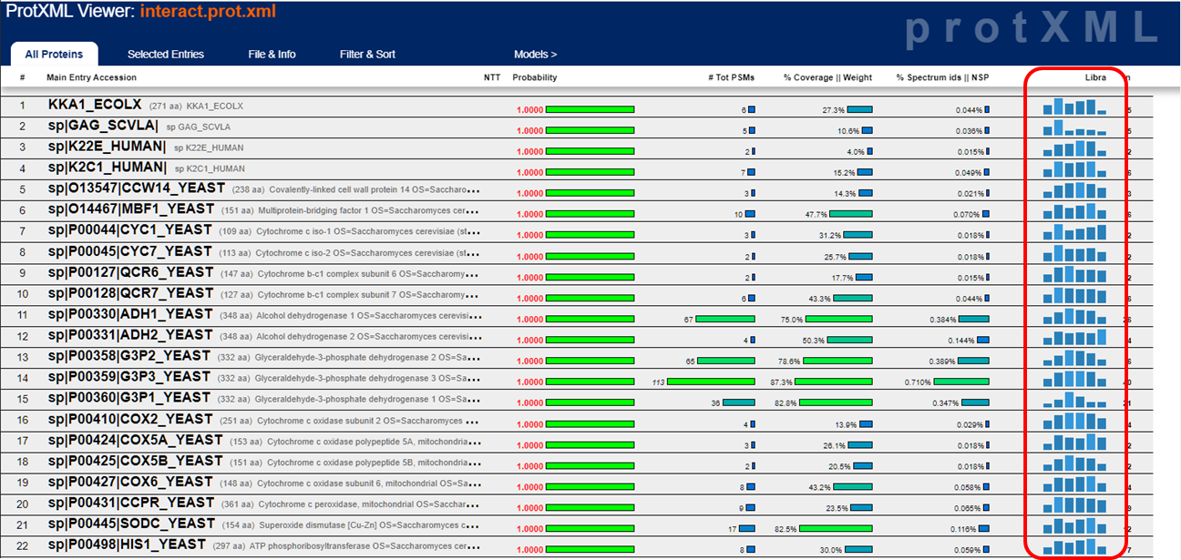
For TMT or iTRAQ labeled samples, the tool that extracts the reporter ion signals is the Libra tool. Assuming the 6-plex TMT reagent was used, the resulting quantitative values are reported as Libra1 through Libra6, corresponding to the reporter ions from 126 through 131. The quantitative peptide and protein values are displayed as below, and the actual values are exported into the tab-delimited text files as described above. Here is the documentation, from back in 2006, that the Libra developers put together describing what it does.

Filtering out contaminants

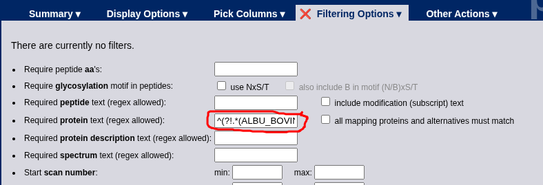
To exclude all 155 contaminants (e.g. trypsin, keratin, albumin) and decoys from the PepXML Viewer, paste the following string into the “Required protein text (regex allowed):” text box of the “Filtering Options” tab. It is one long string with no spaces:

^(?!.*(ALBU_BOVIN|CASA1_BOVIN|CASA2_BOVIN|CAH2_BOVIN|CASB_BOVIN|CASK_BOVIN|CTRA_BOVIN|CTRB_BOVIN|DHE3_BOVIN|LALBA_BOVIN|PEPA_BOVIN|TRY1_BOVIN|TRY2_BOVIN|LYSC_CHICK|OVAL_CHICK|BGAL_ECOLI|ALBU_HUMAN|AMY1A_HUMAN|AMY1B_HUMAN|AMY1C_HUMAN|ANT3_HUMAN|ANXA5_HUMAN|B2MG_HUMAN|BID_HUMAN|CAH1_HUMAN|CAH2_HUMAN|CATA_HUMAN|CATD_HUMAN|CATG_HUMAN|CO5_HUMAN|CRP_HUMAN|CYB5_HUMAN|CYC_HUMAN|EGF_HUMAN|FABPH_HUMAN|GELS_HUMAN|GSTA1_HUMAN|GSTP1_HUMAN|HBA_HUMAN|HBB_HUMAN|HBEGF_HUMAN|IGF2_HUMAN|IL8_HUMAN|INHBA_HUMAN|INHBB_HUMAN|KCRM_HUMAN|LALBA_HUMAN|LEP_HUMAN|LYSC_HUMAN|MYG_HUMAN|NEDD8_HUMAN|NQO1_HUMAN|NQO2_HUMAN|PDGFB_HUMAN|PPIA_HUMAN|PRDX1_HUMAN|RASH_HUMAN|RET4_HUMAN|RS27A_HUMAN|SODC_HUMAN|SUMO1_HUMAN|HARS1_HUMAN|TAU_HUMAN|THIO_HUMAN|TNFA_HUMAN|TRFE_HUMAN|TRFL_HUMAN|UB2E1_HUMAN|UBE2C_HUMAN|K1C26_HUMAN|K2C3_HUMAN|K1C15_HUMAN|K2C79_HUMAN|K2C6B_HUMAN|K1C17_HUMAN|K2C4_HUMAN|K2C73_HUMAN|K2C71_HUMAN|K2C7_HUMAN|K2C8_HUMAN|K1C39_HUMAN|K1C18_HUMAN|K1C28_HUMAN|K1C16_HUMAN|K2C1_HUMAN|K2C5_HUMAN|K2C80_HUMAN|K2C1B_HUMAN|K2C75_HUMAN|K2C6A_HUMAN|K2C72_HUMAN|K1C24_HUMAN|K1C19_HUMAN|K2C74_HUMAN|K1C27_HUMAN|K1C20_HUMAN|K1C9_HUMAN|K1C23_HUMAN|K1C12_HUMAN|K1C14_HUMAN|K2C6C_HUMAN|K1C10_HUMAN|K1C13_HUMAN|K22O_HUMAN|K1C25_HUMAN|K2C78_HUMAN|K22E_HUMAN|K1C40_HUMAN|KRT85_HUMAN|KRT38_HUMAN|KRT34_HUMAN|KRT86_HUMAN|KRT35_HUMAN|KT33B_HUMAN|KRT81_HUMAN|KRT37_HUMAN|KT33A_HUMAN|KRT83_HUMAN|K1H1_HUMAN|KRT82_HUMAN|K1H2_HUMAN|KRT36_HUMAN|KRT84_HUMAN|ALDOA_RABIT|CYC_HORSE|GAG_SCVLA|GFP_AEQVI|K1C15_SHEEP|K1M1_SHEEP|K1M2_SHEEP|K2M1_SHEEP|K2M2_SHEEP|K2M3_SHEEP|KKA1_ECOLX|KRA33_SHEEP|KRA34_SHEEP|KRA3A_SHEEP|KRA3_SHEEP|KRA61_SHEEP|KRB2A_SHEEP|KRB2B_SHEEP|KRB2C_SHEEP|KRB2D_SHEEP|KRUC_SHEEP|LYSC_LYSEN|MYG_HORSE|PEPA_PIG|PEPB_PIG|PEPC_PIG|PLMP_GRIFR|REF_HEVBR|SRPP_HEVBR|SSPA_STAAU|TRYP_PIG|ADH1_YEAST|DECOY_)).*$

Pasted into the filter, it looks like this:

References

1. Empirical statistical model to estimate the accuracy of peptide identifications made by MS/MS and database search. Keller A, Nesvizhskii AI, Kolker E, Aebersold R. Anal Chem. 2002. PubMed link
2. A statistical model for identifying proteins by tandem mass spectrometry. Nesvizhskii AI, Keller A, Kolker E, Aebersold R. Anal Chem. 2003. PubMed link